Register here for next month’s call: Thursday, October 15th 2026, 1 p.m. ET.
Key Takeaways
- Prepayment models continue to track realized speeds well across Fannie, Freddie, and Ginnie collateral, with modeled CPRs running only modestly ahead of actuals
- Non-QM Credit Model 7.1 is getting an October 4th update that broadens the default definition (60+ days delinquent that liquidates = default), roughly doubling measured default rates — though re-estimated severity should offset much of that on a total-loss basis
- The planned “v4.0” prepayment model rebuild has been re-sequenced: an incremental v3.9 release (better FICO/LTV/loan-size controls, FHA/VA accuracy, re-estimated turnover) now comes first, with beta testing in early Q1 2027; the full structural rebuild slides to a Q4 2027 beta
- New deployment options — a Python wheel now in beta, with a REST API/Docker container, Windows DLL, and AWS Batch support to follow — will let clients run RiskSpan’s models inside their own infrastructure, with an MCP/AI connector on the longer-term roadmap
- The Fed funds rate looks set to stay elevated through 2026-2027, the 10-year Treasury is at its highest level since roughly 2007 (~5%), and mortgage rates could push above 7.5% by mid-2027 — a higher-for-longer environment that should keep housing inventory tight but limit the risk of a significant home price decline
This month’s call covered prepayment model back-testing, a deep dive on the model development roadmap (Non-QM Credit Model 7.1, the re-sequenced prepayment model plan, and new deployable model options), and the latest macro and housing picture. Janet Joswick, RiskSpan’s Head of Product, presented in place of Divas Sanwal this month.
You can read the recap below or click here for the entire recording.
Prepayment Model Back-Testing
Modeled CPRs continue to track observed speeds closely across both agency and Ginnie Mae collateral, with model results running only slightly fast versus actuals in the most recent observations. The full interactive backtesting dashboards — with additional cohort and cut options — are available in the RiskSpan platform under RS Insights.
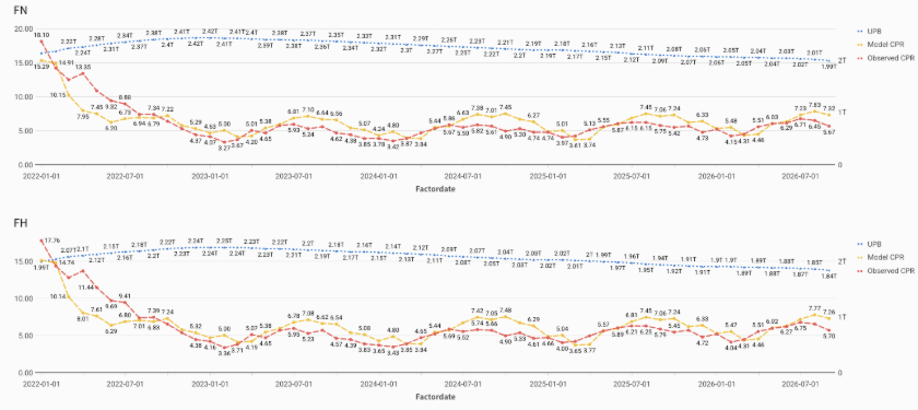
FN/FH WAC 5.5 and Below — Modeled vs. Observed CPR
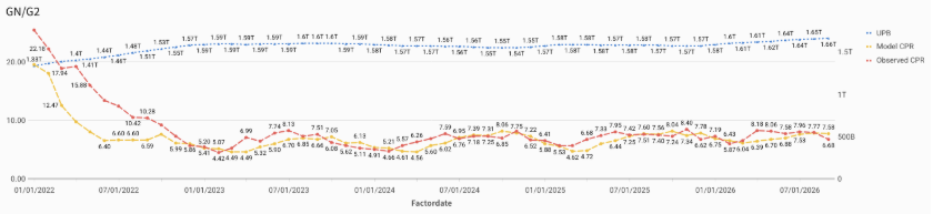
GN/G2 WAC 6 and Higher — Modeled vs. Observed CPR
Model Roadmap Updates
Non-QM Credit Model 7.1
An update to Credit Model 7.1 rolls out on October 4th. The headline change is a simplified default definition: any loan that reaches 60+ days delinquent and liquidates will now be flagged as a default, replacing a more nuanced (but harder to apply consistently) CoreLogic/Cotality-based definition. The change only affects late-stage transition rates (60→90, foreclosure, REO→default), but it roughly doubles measured default rates across documentation types.
Loss severity is being re-estimated in parallel, which is expected to partially offset the higher headline default rate on a total-loss basis — though the team is still working through how to model liquidations straight out of REO, where observed severity is frequently zero. Also landing in this release: prepayment penalty fees will flow through to final cashflows, which matters most for DSCR loans. Securities support for the credit model (currently whole-loan only) is targeted for December.
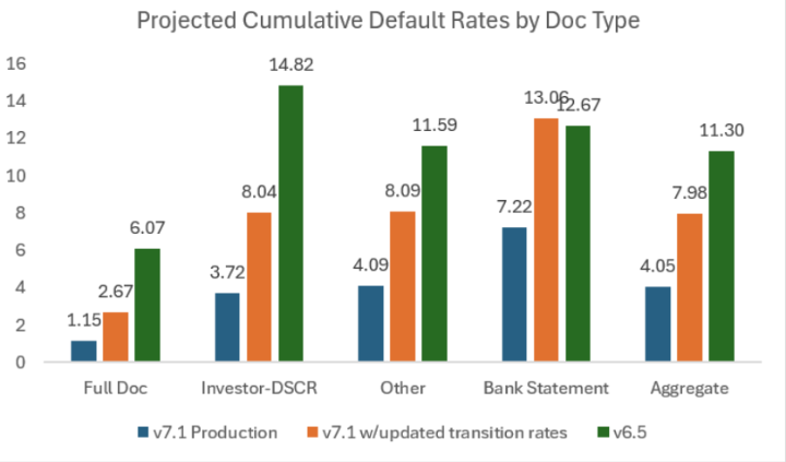
Projected Cumulative Default Rates by Doc Type: v7.1 Production vs. Updated Transition Rates vs. Legacy v6.5
Prepayment Model: Plan Shifted
Based on client feedback, RiskSpan has re-sequenced its prepayment model plans. Rather than moving straight to the full structural rebuild originally envisioned as v4.0, a faster, incremental v3.9 release will come first, building on the existing 3.8 agency model. Key improvements include additional FICO/LTV/loan-size controls, better floor and override controls, improved FHA-vs-VA accuracy within the Ginnie model (a frequent client pain point), and re-estimated turnover using post-COVID and recent jumbo-loan data. Beta testing is targeted for early Q1 2027, with full production shortly after.
The larger structural rebuild — now positioned as v4.0, with dedicated sub-models for curtailment, buyout, and cash-out — is still planned, with beta testing now targeted for Q4 2027 and production release in H1 2028. Clients interested in the v3.9 beta are encouraged to reach out to the RiskSpan team.
Deployable Model — Coming to Beta
RiskSpan is piloting a standalone, deployable version of its models for clients who want to run them inside their own infrastructure rather than through the platform UI or API. First out: a Python wheel (pip-installable, no server or network hop), already in beta with one client. On the roadmap: a REST API/Docker container, a Windows DLL for native C/C++ integration, and AWS Batch support. Further out, RiskSpan is also exploring an MCP connector that would let users run projections and calibrations conversationally through Claude or other AI tools, without writing code. Clients with use cases for model access outside the platform are encouraged to reach out.
Macroeconomic Update
The Fed funds rate is expected to stay elevated, with CME FedWatch data showing the current 375–400 bps range likely moving to 400–425 bps by year-end; a rate cut looks unlikely through 2026–2027.
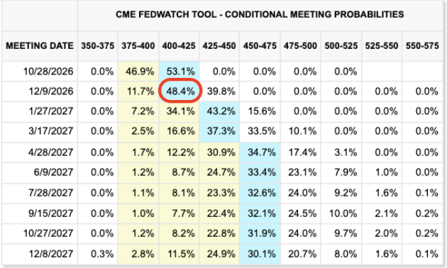
CME FedWatch Tool — Conditional Meeting Probabilities
The Treasury curve has shifted up in an almost parallel move over the past month, with the 10-year around 5% — its highest level since roughly July 2007.
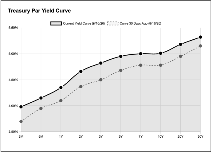
Treasury Par Yield Curve: Current vs. 30 Days Prior
Market consensus forecasts have the 10-year Treasury climbing above 5.4% in 2027, with 30-year mortgage rates potentially exceeding 7.5% by mid-2027. Mortgage rates have already moved sharply higher in recent weeks, with Mortgage News Daily quoting 7.24% as of September 16th.
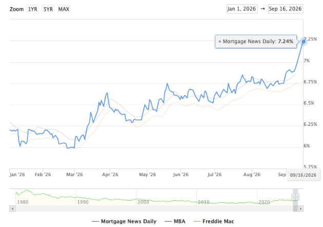
30-Year Fixed Mortgage Rate, Trailing 2 Years (Mortgage News Daily / MBA / Freddie Mac)
For housing, the combination of persistently high rates, negative homebuilder sentiment (fewer housing starts, less incentive spending), and low existing-home inventory — owners remain reluctant to give up lower-rate mortgages — should keep turnover and supply constrained.
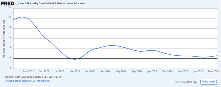
S&P Cotality Case-Shiller U.S. National Home Price Index, YoY % Change
RiskSpan’s view: that inventory scarcity should limit the risk of a significant home price decline, even as affordability stays stretched and core inflation remains elevated despite continued Fed intervention.
We continue to add additional analytics reports on the RiskSpan Platform. Please visit www.riskspan.com to request access.
As always, please feel free to contact us to discuss or learn more.
A Case Study for Mortgage Investors
If the answer is developer hours saved, I think we’re measuring the easy part — and missing the bigger prize.
The problem isn’t information. It’s acting on it.
The information an investor needs mostly exists already. It just arrives scattered — emails, dealer commentary, internal reporting, a dozen data feeds. Tracking all the sources is hard enough. Deriving insight and acting on it in time? Nearly impossible at human speed.
The first-order ROI is real — and one-time
Yes, AI automates the collection. Yes, AI coding tools can stand up the dashboard that aggregates everything, with drill-downs. That’s real ROI, and worth capturing. But it’s one-time ROI: the savings recur, but the capability doesn’t compound. Your highest-value people are still going through the motions: clicking, drilling, hunting for the missing piece, deciding what to look at next.
The durable ROI is different
It comes from making the high-value portfolio manager (PM) and the uber-analyst more powerful. Not summaries — actions: sharper pricing, less leakage through better risk management, new sources of return spotted as market conditions evolve.
The tech world calls the machinery “loops enhanced by graph engineering.” Strip the jargon and it’s simple: workflows that manage dependencies and put human validation gates at the decision points. Software developers have been working this way for months — sometimes without naming it. The processes translate to investing better than you’d expect.
Two properties do most of the work.
First: the graph
The workflow maps which tasks actually depend on which. Everything independent runs in parallel — that’s speed. Results synchronize before a decision is staged — that’s fewer half-formed questions thrown back at you. The PM gets one decision point with the evidence assembled, not twenty interruptions.
Second — and this is the part I find most interesting: unknown unknowns
Newer models can reason much longer and more carefully than the last generation, and one consequence is underappreciated: they are effective at surfacing gaps in your own framing. There is a specific class of unknown unknowns — things well-represented in the model’s knowledge but outside yours — that a model can convert into explicit questions. You’re watching delinquencies by geography; it asks whether insurance-premium shocks in those same markets belong on the dashboard. You benchmark refi incentive to a survey average; it asks what lenders are actually offering that borrower today.
That’s a genuine and valuable capability. Here’s the trap: believing that a “what am I missing?” pass gives you coverage. It doesn’t. Run it ad hoc and you get a different, unaudited coverage claim every time.
So we use the capability where it belongs — at design time. When we build a loop, human and AI iterate on what the loop should watch, and the blind spot questions get argued out once, deliberately, by people who know the portfolio. Then the answers are committed to a deterministic pipeline: the same checks, every run, written down. Coverage becomes explicit and auditable — not an assumption remade on every prompt. And when something does slip through, it doesn’t just get fixed; it becomes a permanent regression test the system must pass forever.
Coverage compounds. That’s the difference between a workflow and a chat window.
What this looks like in practice
We started with non-QM (non-qualified mortgage) investors. The loops we’re building:
- Pricing — wholesale rate sheets parsed daily; every program and pricing change diffed against the market
- Market intelligence — new deals scored rich or cheap — over- or underpriced — vs comparables the day they price; street commentary attributed to its source and date, never blended into an unattributed consensus
- Asset allocation — where return is migrating as conditions evolve: primary vs secondary market, cohort vs cohort
- Risk & outliers — roll rates (how delinquencies migrate from 30 to 60 to 90 days late), concentrations, and the checks that separate borrower credit deterioration from a soft local housing market
- News & regulatory scanners — policy, litigation, counterparty watch, with two independent sources behind any credit-negative claim
- Macro — the weekly backdrop every other loop cites, so context is shared instead of re-derived
Case study: a mortgage investor’s morning in the pricing loop
Here’s one of those loops in the wild — a demonstration run on live market data from this August.
A non-QM investor’s earliest view of the primary market lives in wholesale rate sheets: nine lenders in this build, each publishing rate grids and adjustment matrices in its own format, on its own schedule. Read together, they’re a running record of who wants what risk at what price. Almost nobody reads them together. The realistic before-state isn’t a team parsing nine sheets every morning — it’s an analyst spot-checking two or three when a deal is in play, and everything else surfacing weeks later, if at all.
The loop runs before the market day starts. It fetches and parses every sheet, then works as a graph: nine lenders in parallel, every price cell and every adjustment diffed against that lender’s own history, results synchronizing only where the analysis genuinely needs all nine — cross-lender dispersion, and the comparison against where benchmarks moved. All arithmetic runs in SQL against the loaded data, never inside the model, and every number keeps a link back to the exact source file it came from. That morning: 20,000+ data points scanned.
What reached the PM was not 20,000 data points. The gates — freshness checks, numeric reconciliation, materiality thresholds, an independent model challenging the findings — cut it to six candidate findings, of which five survived the challenge — two material signals and three escalations — staged as a single review that took about fifteen minutes. The diagram below shows that morning end to end.
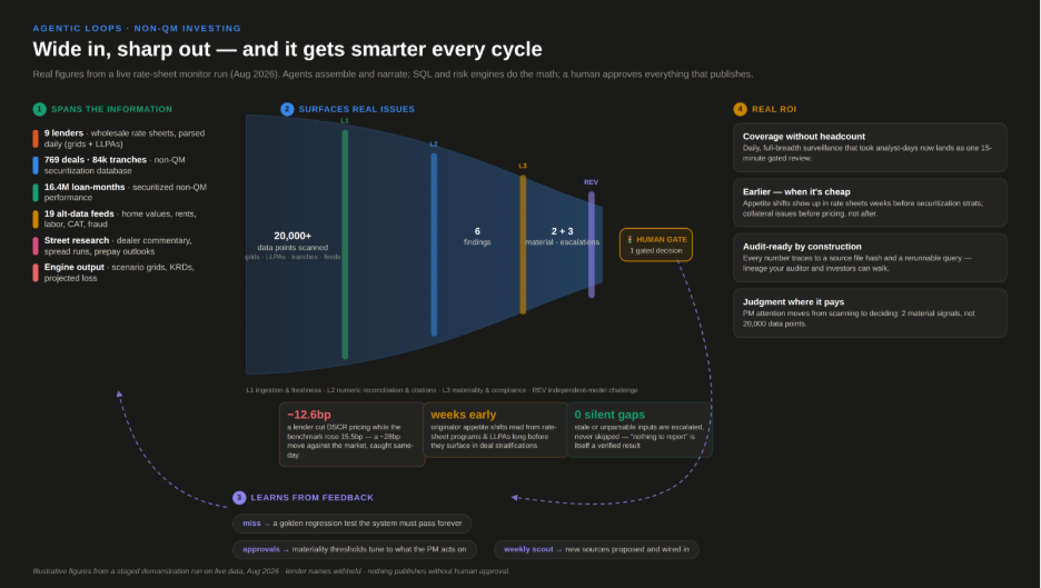
The material catch: one lender had cut pricing on DSCR loans (investor-property loans underwritten on rental cash flow) by 12.6 basis points (hundredths of a percent) the same morning benchmark mortgage rates moved 15.5bp the other way — roughly a 28bp swing against the market, caught same-day. That’s valuable twice. Tactically, it’s better information for anyone pricing or bidding that collateral this week. Strategically, it’s an appetite signal: an originator reaching for volume shows up in its rate sheet weeks before it shows up in the collateral of the deals you’ll be offered. Wait for the deal stratifications — the collateral tables published when a deal comes to market — and you’re reading old news.
The three escalations matter just as much. Three of the nine sources came in stale or unparsable that morning, and the loop escalated them instead of skipping them — so “nothing new from the other six” is a verified statement, not an assumption. That’s the unglamorous half of the ROI: gates are what keep silent gaps from quietly turning your coverage claim into fiction.
The ledger for that single morning: full-breadth coverage that used to cost analyst-days, delivered as a fifteen-minute gated review. A signal in hand weeks earlier than the alternative. An audit trail your risk committee — or your investors — can walk from any number back to a source file and a rerunnable query. And the PM’s judgment spent on two decisions, not twenty thousand data points.
The loop part matters most: every approval or correction at the gate tunes what the system treats as material, and every miss becomes a new golden test. It gets smarter every cycle.
So how do we measure the ROI?
- Headcount the PM would have needed — sure, but that one’s overdone
- Basis points of better pricing across the book — what would 1bp be worth in yours?
- The wrong decision you didn’t make — the fraud flag or the stale input caught before anything was priced off it
- And the verification gates themselves. Unchecked AI doesn’t produce zero ROI; it can produce negative ROI. The gates are what keep the sign positive.
How are you measuring yours? What’s the decision in your process that arrives too late today?
If you’re building toward something similar — or stuck in dashboard land — please message me. Happy to compare notes.
Register here for next month’s call: Thursday, September 17th 2026, 1 p.m. ET.
Key Takeaways
- Prepayment models continue to track realized speeds well, even as July speeds fell across the board: roughly 4% for FN/FH coupons 5.5 and below, 3.8–4.7% for FN/FH 6 and higher, and 1.7% (≤5.5) and 7.5% (6+) for Ginnie
- A deeper look at the conventional universe shows where the v3.7 model is straining: it ran 1.7 CPR fast on FH30 in July (10.0 modeled vs. 8.3 actual), missed month-over-month direction for out-of-the-money cohorts, and shows S-curves that are too flat for unseasoned loans and too steep for seasoned ones
- Federal debt has reached $40 trillion (about 125% of GDP, with a deficit near 6% of GDP), while consumer stress is concentrated in credit cards (~13% of balances 90+ days delinquent), autos (approaching 6%), and borrowers aged 70+
- The 30-year Treasury touched 5.30%, its highest level in roughly 20 years; the Fed funds rate (350–375 bps) is expected to hold at the next two meetings, with a meaningful chance of an increase and no cuts expected through 2027
- Consensus forecasts put the 10-year Treasury above 5% in 2027 and 30-year mortgage rates above 7% around the turn of the year; with core inflation near 2.5%, a weakening labor market, and tight inventory, home prices look more likely to stagnate than fall significantly
This month’s call covered prepayment model back-testing, a conventional deep dive on model performance and CBR/CCR trends, federal and consumer debt, and the latest macro and housing picture. Yashwant and Anish Roy of RiskSpan’s quantitative modeling team and Divas Sanwal presented.
You can read the recap below or click here for the entire recording.
Prepayment Model Back-Testing
Modeled CPRs continue to track observed speeds closely, though speeds declined across all cohorts with the August factor data update. Fannie/Freddie coupons 5.5 and below fell approximately 4%. For coupons 6 and higher, Fannie speeds fell 4.7% and Freddie 3.8%. Ginnie Mae coupons 5.5 and below fell approximately 1.7%, while Ginnie 6 and higher fell approximately 7.5%.
The team attributes the slowdown in premium coupons (6 and higher) primarily to a 7 bp rise in the driving mortgage rate, partially offset by a 5% increase in day count. For coupons 5.5 and below, the decline reflects an 8% month-over-month drop in seasonal housing turnover. The full interactive back-testing reports are available in the RiskSpan platform.
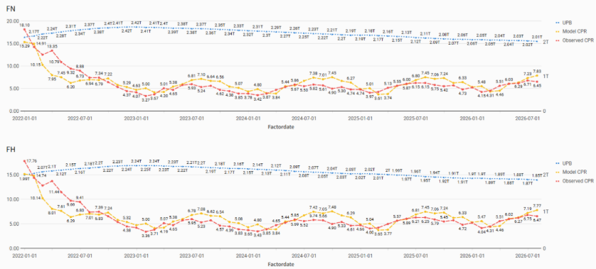
FN/FH WAC 5.5 and Below — Modeled vs. Observed CPR
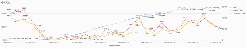
GN/G2 WAC 6 and Higher — Modeled vs. Observed CPR
Conventional Deep Dive: Model Performance and CBR/CCR Trends
As in prior months, the quantitative modeling team took a closer look at the conventional universe using model v3.7. This research also supports the next-generation prepayment model initiative by providing a more granular view of prepayment behavior and highlighting opportunities for future enhancements.
FH30 Aggregate and Coupon-Level Speeds
FH30 printed 8.3 CPR in July 2026 versus a model prediction of 10.0 CPR, a fast bias of 1.7 CPR. Month over month, actual speeds fell 4% while model speeds rose 4%. Following client feedback, the team added 3-, 6-, and 12-month error ratios this month. At the aggregate level, the model carries a 12% fast bias over the trailing three months, versus only 2% over six and twelve months. Over the trailing 12 months, coupons 1.5%–5.5% have been persistently about 10% faster than actuals, while coupons 6.0%–7.0% have been persistently about 10% slower.
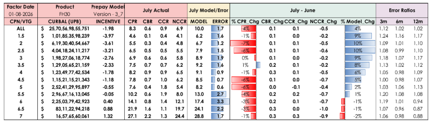
FH30 Aggregate and Coupon-Level Speeds — Actual vs. Model v3.7 (July 2026)
Missed Directionality for Out-of-the-Money Cohorts
The model missed month-over-month direction for out-of-the-money cohorts: model speeds rose about 7% while actuals fell about 3%. In-the-money cohorts behaved as expected, with model speeds down 1% and actuals down 2%. The team believes the miss is driven by the model’s seasonality component, which needs further calibration. Level errors are largest on the higher, in-the-money coupons, but month-over-month sensitivity is greater for out-of-the-money cohorts. Behind the aggregate 4% decline in actual speeds, the 7 bp rise in the 30-year driving rate and 8% drop in turnover seasonality were partly offset by a 5% increase in day count.
S-Curves by Loan Size and Seasoning
New this month, the team plotted S-curves of actuals against the model by loan size and moneyness, split into unseasoned (WALA 0–18, left) and seasoned (WALA 18–60, right) loans. The findings point in opposite directions:
- Unseasoned loans: the model S-curve is too flat. The in-the-money $400K+ cohort has a significant slow bias of about 12 CPR at a 7% coupon. Out-of-the-money cohorts converge within about 5 CPR, except the $0–200K cohort, which runs about 10 CPR slow. The model also does not capture the expected rise in speeds with loan size at a given incentive.
- Seasoned loans: the model S-curve is too steep. The in-the-money $400K+ cohort has a fast bias of about 7 CPR at a 7% coupon, and the $0–200K cohort is about 5 CPR fast. The model did not apply enough burnout decay.
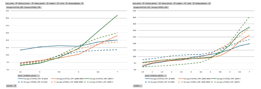
FH30 vs. Model (v3.7) S-Curve by Loan Size — Last 3 Months, WALA 0–18 (L) vs. 18–60 (R)
Buyout and Curtailment Across the Coupon Stack
Curtailment (CCR) follows a hump shape across coupons, peaking around 5.5%. This is primarily a seasoning effect: the 5.5% cohort has the lowest WALA, curtailment is front-loaded and peaks around a WALA of four, and the pattern is amplified by occupancy and purpose mix. Buyout (CBR), by contrast, rises sharply with coupon, especially at the high end. At a 7% coupon, CBR is roughly 3–5 times that of lower coupons, and the 7% coupon also has the lowest average FICO in the stack (725), consistent with higher-coupon loans being disproportionately associated with borrower credit stress.
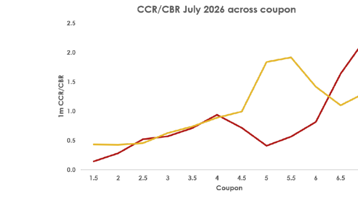
FH30 CBR and CCR Across Coupon (Actual), July 2026
Debt and Consumer Credit
The call opened this section with a new milestone: total U.S. national debt has reached $40 trillion. Roughly $50 trillion is expected within about five years, which RiskSpan’s reference thresholds treat as the point at which federal debt becomes unsustainable.
| Federal Metric | Current (Aug 2026) | Unsustainable Threshold |
| Total National Debt | $40 trillion | ~$50T by 2031 |
| Debt-to-GDP Ratio | 124.6% (June) | 140% (Penn Wharton) |
| Federal Budget Deficit | ~6% of GDP | 4–5% unsustainable |
| Deficit/Revenue Ratio | $1.33 spent per $1 revenue | $1.20+ unsustainable |
Federal Government Debt vs. Reference Thresholds
Federal interest costs are a growing concern. With the 30-year Treasury at 5.30%, new issuance replaces older, cheaper debt at higher rates, and debt service is already the government’s second-largest expense after Social Security. Unlike Social Security, it cannot be cut without risking the country’s credit rating.
Household debt stands at approximately $18.77 trillion, up about 2.1% year over year (and essentially flat versus $18.78 trillion in Q1, per the NY Fed’s August report). Mortgages make up about $13.6 trillion of that, leaving roughly $5 trillion of non-mortgage debt, with the fastest growth in auto loans and credit cards.
| Debt Category | Amount | % of Total | YoY Growth |
| Total Household Debt | $18.77T | 100% | ~2.1% |
| Mortgage Debt | $13.58T | 72.3% | ~2.0% (all-time high) |
| Auto Loans/Leases | $1.72T | 9.2% | 2.9% |
| Credit Cards | $1.26T | 6.7% | 3.9% |
| Student Loans | $1.87T | 9.9% | Slowed with payment pause |
| Other | $0.4T | 2.1% | Varies |
Household Debt Breakdown, Q2 2026
Where the Stress Is Showing
- Credit cards: There are approximately 650 million credit card accounts, roughly three per adult, and the count has grown rapidly over the last decade while other account types have been flat. Card balances of about $1.3 trillion sit against roughly $5.5 trillion in limits (about 20% utilization), and approximately 13% of balances are 90+ days delinquent, close to the financial-crisis peak. Much of this delinquent balance sits with smaller banks and fintechs rather than large banks, which have been careful about extending credit to lower-credit borrowers.
- Auto loans: 90+ day delinquency is approaching 6%, higher than at any point during the financial crisis. With the used-car market where it is, servicing and even repossession are often unprofitable, which is a concern for lenders as well as borrowers.
- HELOCs: Home equity revolving balances have grown meaningfully over the last four years, with about $0.5 trillion drawn against roughly $1 trillion in limits (about 50% utilization).
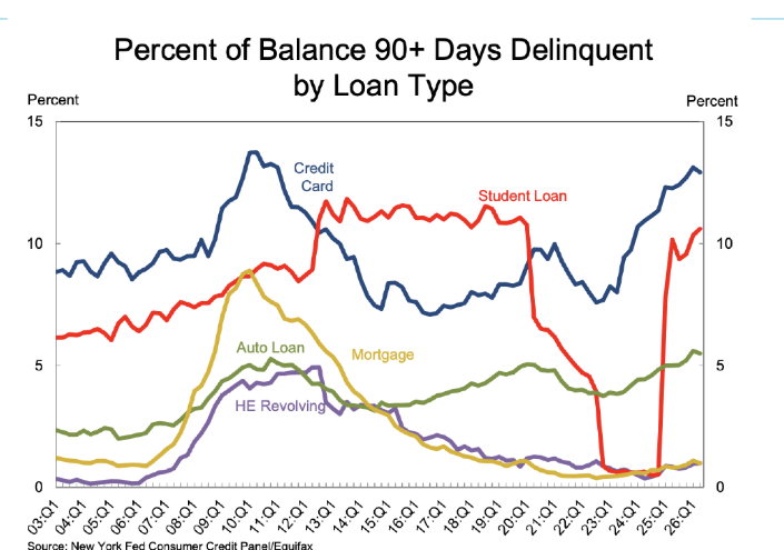
Percent of Balance 90+ Days Delinquent by Loan Type (NY Fed Consumer Credit Panel/Equifax)
One notable finding in the NY Fed data: younger borrowers have always shown the highest delinquency transition rates, but the 70+ age group now stands out for auto loans and credit cards, with rising transitions into serious delinquency. These borrowers are often on fixed incomes, so RiskSpan views this as an indirect signal of how inflation is eroding households’ ability to maintain their lifestyles.
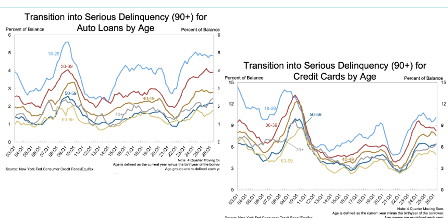
Transition into Serious Delinquency (90+) by Age — Auto Loans (L) and Credit Cards (R)
Where Averages Deceive
The average hides a sharp split in debt burden. The illustrative comparison below shows how much the mix of debt matters: a median household’s debt is dominated by low-rate mortgages, while the bottom quartile carries disproportionately high-rate revolving and subprime debt. Any economic shock could have an outsized impact on the credit market through that bottom segment.
| Median Household | Bottom Quartile | |
| Gross income | ~$80,000 | ~$40,000 |
| Disposable income | ~$65,000 | ~$35,000 |
| Debt | ~$35,000 | ~$15,000 |
| Debt mix | Low-rate mortgage (3.5–4%), card balance (~20%), auto loan (~8%), student loans | Subprime auto (~12%), credit cards (~24%), medical debt |
| Debt burden (% of disposable income) | ~30–35%: stretched but managing | 40–50%: severely strained |
Median Household vs. Bottom Quartile (Reference Figures)
Macroeconomic Update
Rates
The Fed made no change to the Fed funds rate in July and does not meet in August. The current range is 350–375 bps, and CME FedWatch data point to a hold in September (about 67% probability), a year-end range of 375–400 bps, and a meaningful likelihood of an increase this year. A rate cut looks unlikely through 2026–2027.
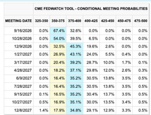
CME FedWatch Tool — Conditional Meeting Probabilities
On the Treasury side, the Treasury curve (Aug 17–18) showed the 2-year at 4.19%, 5-year at 4.36%, 10-year at 4.72%, and 30-year at 5.30%, the highest 30-year yield in roughly 20 years.
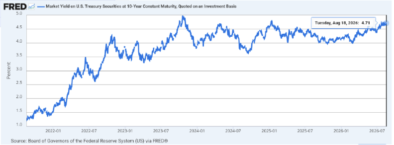
10-Year Treasury Constant Maturity Yield (FRED)
Market consensus has the 10-year Treasury moving above 5% in 2027, and 30-year mortgage rates rising above 7% around the end of this year or early 2027, peaking near 7.2%. Mortgage rates dipped just below 6% in late February, but have since climbed to roughly 6.75–6.80% (Mortgage News Daily), and the consensus path suggests more room to rise before they fall.
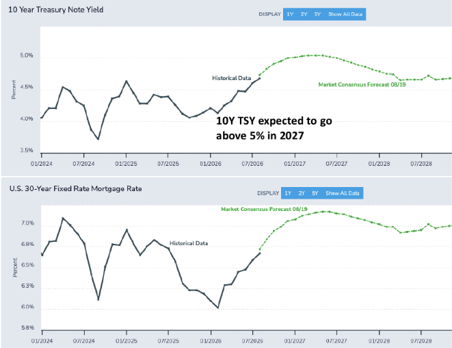
10-Year Treasury and 30-Year Fixed Mortgage Rate — Market Consensus Forecast (as of 8/19)
Inflation, Growth, and Labor
Core inflation has sat around 2.5% for a long time, well above the Fed’s 2% target. Much of the recent volatility in headline inflation, which peaked near 4.2% in May before easing to 3.5% in June and 3.4% in July, has been driven by energy prices. With core measures still elevated, the Fed has little flexibility to cut. The Producer Price Index is also rising, a signal of higher consumer inflation in the coming months, since retailers have limited capacity to absorb further cost increases.
| Inflation Measure | July 2026 | June 2026 | Fed Target |
| CPI (Headline) | 3.4% YoY | 3.5% YoY | 2.0% |
| Core CPI (ex-food/energy) | 2.5% YoY | 2.6% YoY | ~2.0% |
| PCE (Headline) | 3.2% YoY (est.) | 3.3% YoY | 2.0% |
| Core PCE (ex-food/energy) | 2.6% YoY (est.) | 2.7% YoY | 2.0% |
| Energy Component | Fell 5.7% MoM | Up 15.7% YoY | N/A |
Headline vs. Core Inflation
On growth, current estimates put 2026 GDP growth at around 2% (Goldman Sachs at 2.8%, Deloitte at 2.0%), with 2027 expected to be weaker, and Deloitte’s downside scenario is recessionary. The labor market is showing strain: July nonfarm payrolls fell by 23,000, a first-time decline, and June was revised down sharply to +20,000. Unemployment ticked down to 4.1%, but only because labor force participation also fell to 61.4%, and with wage growth slowing to 3.2%, real wages are now negative.
| Labor Market Metric | July | June | Change |
| Nonfarm Payrolls | -23,000 | +20,000 (revised) | -43,000 |
| Unemployment (U-3) | 4.1% | 4.2% | -0.1pp |
| Labor Force Participation | 61.4% | 61.5% | -0.1pp |
| Wage Growth (YoY) | 3.2% | 3.5% | -0.3pp |
| CPI Inflation (YoY) | 3.4% | 3.5% | -0.1pp |
| Real Wage Growth | -0.2% | 0.0% | -0.2pp |
Labor Market, July 2026
Implications for the Housing Market
The Case-Shiller National Home Price Index is still growing, but only about 1% year over year. Persistently high mortgage rates mean little refinance activity, and out-of-the-money loans are likely to stay that way. Homebuilder sentiment has turned negative as costs rise and margins look thin, so housing starts are expected to decline. Builder incentives such as down payment help and rate buydowns, which have supported a significant share of new-home sales in recent years, are coming under pressure.
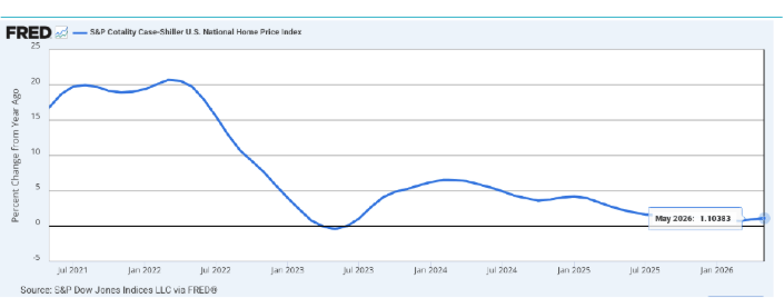
S&P Cotality Case-Shiller U.S. National Home Price Index, YoY % Change
RiskSpan’s view: with few new homes available and builder incentives fading, inventory constraints make a significant home price decline unlikely. Prices should stay close to current levels, with perhaps a moderate increase. Geopolitics remains the major macro driver of markets, so it is worth keeping an eye on.
We continue to add additional analytics reports on the RiskSpan Platform. Please visit www.riskspan.com to request access.
As always, please feel free to contact us to discuss or learn more.
Register here for next month’s call: Thursday, August 20th, 2026, 1 p.m. ET.
Key Takeaways
- Prepayment models remain reliable, but the fast bias showing up in in-the-money cohorts is worth watching if rates keep climbing and more loans move into the money
- Non-QM credit risk is becoming a bigger focus right as CM 7.1 goes live — the model is arriving just as delinquency trends turn less benign
- The market has flipped from pricing rate cuts to pricing a hike this year — a real shift in the rate outlook, not noise
- Elevated rates and mortgage costs look like a multi-year reality rather than a temporary plateau, with labor data adding a note of underlying softness beneath a falling headline unemployment rate
This month’s call covered prepayment model back-testing, a deep dive on conventional model performance, the growing Non-QM universe, the production release of RiskSpan’s Non-QM Credit Model (CM 7.1), and the latest macro picture.
You can read the recap below or click here for the entire recording.
Prepayment Model Back-Testing
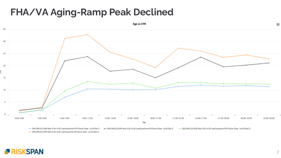
The prepayment model continues to closely track realized speeds across Fannie, Freddie, and Ginnie collateral. Discount coupons (WAC 5.5 and below) remain structurally low and range-bound at roughly 4–8 CPR, consistent with these loans sitting out of the money in a turnover-driven regime. Premium coupons (WAC 6 and above) eased slightly in June, as a 13 bp increase in the driving mortgage rate outweighed a 5% rise in day count — visible in a modest month-over-month flattening of the conventional S-curve. FHA/VA aging-ramp peaks have also come down from prior levels, with VA loans continuing to ramp faster and higher than FHA.
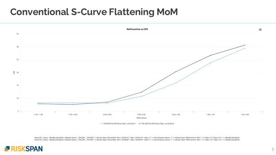
Conventional S-Curve Flattening MoM
FHA/VA Aging-Ramp Peak Declined
Conventional Deep Dive
A closer look at FH30 and FN30 performance found the model running fast versus actuals in June — a bias of roughly 1 CPR — with month-over-month direction captured well but magnitude off: the model overreacts in out-of-the-money cohorts and underreacts in in-the-money cohorts, where its error is markedly larger (~2 CPR vs. ~0.8 CPR).
Curtailment and buyout activity move in opposite directions over a loan’s life. Curtailments are front-loaded, peaking in the newest vintages and fading with age, while buyouts build slowly and grow as loans season and credit stress accumulates. The effect is large: comparing 2023 to 2025 vintages in higher-coupon cohorts, Freddie Mac loans show roughly 7x the buyout activity, and Fannie Mae loans show roughly 3x.
Non-QM Universe and Credit Model 7.1
Non-QM issuance is tracking toward roughly $100B for 2026 — Q2 came in around $27B, down 16% quarter-over-quarter but up 58% year-over-year — with originations running at about $170–180B. Delinquency data gave a mildly encouraging signal, with the 2023 vintage appearing to plateau around 24 months of loan age, though risk stays concentrated in bank-statement and self-employed borrowers and lower FICO bands. Zooming out, delinquency has been climbing across consumer credit broadly (subprime auto, personal loans, mortgage, Non-QM) since 2021.
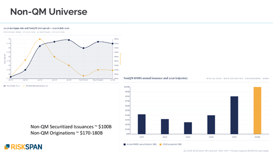
Non-QM RMBS Issuance and 2026 Trajectory
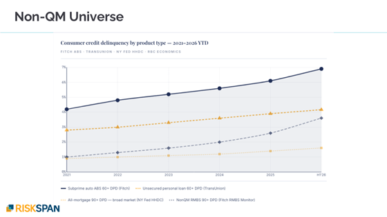
Consumer Credit Delinquency by Product Type
Against that backdrop, RiskSpan’s Non-QM Credit Model — CM 7.1 — has moved into production and is now available to all clients. It runs four independent transition models by documentation type (Bank Statement, DSCR, Full Doc, Other), feeding into a single liquidation-timeline and severity model recalibrated to current Non-QM performance.
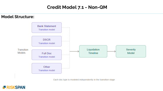
CM 7.1 Model Structure
Macroeconomic Update
The biggest change this month is at the Fed. A couple of months ago the market was pricing in up to two rate cuts this year; CME FedWatch data now show meaningful odds of a hike instead, with the Fed funds rate seen moving from 350–375 bps toward 375–400 bps by year-end.
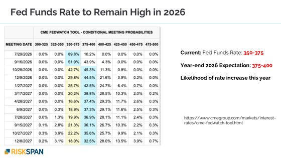
Fed Funds Rate to Remain High in 2026
Longer rates have followed suit. The 10-year Treasury, just above 4.5%, is expected to climb another 20–25 bps toward ~4.9% before easing — but to hold above 4% for a couple of years. Mortgage rates, currently around 6.5–6.6%, are expected to reach as high as ~6.9% by spring 2027 and stay above 6.5% for the next two to three years.
The labor market sent a mixed signal. June payrolls rose just 57K, roughly half of what was expected, and April/May were revised down a combined 75,000 jobs — pointing to real underlying softness. Headline unemployment actually ticked down to 4.2%, but that came from falling labor force participation (61.5%, the lowest since 2021) rather than hiring; the household survey showed 507,000 fewer people employed. On a brighter note, CPI eased to 3.5% year-over-year and wage growth matched it exactly — the first time in 12–18 months that real wage growth hasn’t been negative.
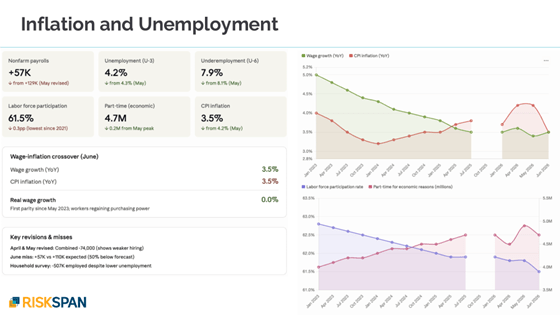
Inflation and Unemployment

We continue to add additional analytics reports on the RiskSpan Platform. Please visit www.riskspan.com to request access.
As always, please feel free to contact us to discuss or learn more.
My first Wall Street job as a junior programmer was to process pool tapes from the GSEs and Ginnie Mae. Every month, the tapes arrived and an operator loaded them. Then I ran through a series of scripts — the same series, in the same order — to produce prepayment reports. The reports were printed, photocopied, stapled. Every desk got its copy before the open. For this, the firm paid me slightly more than the prevailing minimum wage.
This went on for a couple of years. Eventually two things happened: I wanted to get paid more, and management decided I could do more useful things — like help build prepayment and OAS models. My boss’s solution was not to hire another me. It was to automate the whole process with proper error handling and hand it off to the operator who was already running other overnight jobs.
Looking back, the strange part isn’t that the job got automated. It’s that for two years, nobody thought it was odd to pay a human to be a scheduler. The job was never “Suhrud runs the reports.” The job was “the reports get run.” The moment someone articulated it that way, the answer was obvious.
I’ve been thinking about this a lot lately, because the industry is busy making the same mistake with a much more expensive employee.
The rerun
Today we wire LLMs into our systems through connectors and MCP servers, and then we ask them to perform recurring tasks. Pull the latest remittance data. Run the QC checks. Format the surveillance report. Post it to the channel. Every day. Sometimes every hour.
Here’s what actually happens on each run: the model re-reads its instructions, re-loads its tool definitions, rediscovers the schema, re-reasons through steps it reasoned through yesterday, and re-derives the entire task from first principles. It is me in that back office — except the photocopier bills by the token, and the junior programmer occasionally hallucinates a column mapping.
That is the junior programmer problem: an LLM is a bright, expensive generalist being asked to do clerical work on repeat. It can help figure out the process, draft the checklist, and handle exceptions. But if the job is the same every morning, the goal should be to convert the junior programmer’s reasoning into reviewed code and let the system run it. The junior programmer belongs at the design table and the exception desk — not standing at the photocopier forever.
Two problems compound here. One is cost. The other, worse one, is that the junior programmer is non-deterministic.
The economics
Take a realistic daily agentic job: a report run against a data warehouse via MCP connectors, with QC checks and a written summary.
Each turn carries a base context of roughly 20K tokens — system prompt, tool definitions, instructions. The agent makes maybe 15 tool calls (list the tables, query, check, query again), each returning a few thousand tokens of results. Because every turn re-sends the growing conversation, cumulative input compounds to roughly 800K–850K input tokens per run, plus a few thousand tokens of output.
At current mid-tier model pricing (about $3 per million input tokens, $15 per million output), that’s roughly $2.50 to $2.75 per run. Daily across 22 business days: ~$55 to $60 a month. For one report. Run thirty recurring jobs like that — not an unusual number for a surveillance or analytics desk — and you’re around $1,700 a month for work that is identical every day.
Now the honest version, because a sophisticated reader will raise it immediately: prompt caching cuts repeated input cost by about 90%, and batch APIs knock another 50% off. A well-engineered agent run might land closer to $0.30–0.50, or roughly $10 a month per job. That’s real, and if you’re going to keep agents in the loop, you should absolutely use both.
But compare the alternative. A scheduled script on Cloudflare Workers runs free or nearly so. AWS Lambda executes this class of job for well under a dollar a month. And the one-time cost of having the LLM write that script? Maybe $1–5 of tokens. Even against the fully optimized agent, the deployed script is one hundred to a thousand times cheaper than the agent — and that gap is before you price the risk.
The overconfidence risk (AI hallucination) is worse than the bill
A deployed script is deterministic and auditable. Same inputs, same outputs. It’s versioned, diffable, and reviewable. When it breaks, it breaks loudly and identically.
An LLM performing the task fresh each morning is a new draw from a distribution. It will usually do the right thing. Occasionally it will skip a QC check, misread a schema change as an instruction, or format a number differently on run 47 — silently. In regulated finance, “the agent usually gets it right” is not a control. Anyone who has sat through a model governance review knows that the question isn’t whether the process works; it’s whether you can prove what it did, every time.
To be fair, this argument cuts both ways, and pretending otherwise would be dishonest. LLM-generated code can also be wrong — subtly, in edge cases, in ways that survive a casual glance. The principle isn’t “code good, agent bad.” The principle is review once, run many. A script gets one round of concentrated human scrutiny, and that scrutiny amortizes across thousands of executions. An agent-in-the-loop asks you to trust a fresh, unreviewed performance every single run. My boss didn’t just automate my job — he automated it with error handling, and someone reviewed that logic before the operator ever touched it. That review was the whole point.
Use the LLM for Judgment, Not Execution
The obvious objection is that nobody serious should run a fully deterministic job through an agent loop. Fair. But many tasks are not purely deterministic. They look repetitive on the surface while still containing moments of judgment: triaging anomalies, deciding whether a failed reconciliation is a data problem or a real signal, or writing the two sentences of commentary that make a report useful. Those are legitimate places for an LLM.
But that does not make the LLM the operator.
The right pattern is LLM as designer, author, and escalation point — not as the thing that runs the job every day. The operating layer should be code: scheduled, versioned, reviewed, monitored, and boring. Code should extract the data, validate it, compute the results, apply the rules, and distribute the output. The LLM should be called only when the process reaches a judgment node: when a check fails, when a number looks strange, when the rules do not cover the case, or when a human-quality narrative is actually needed.
That is the same pattern my boss landed on in the 1990s. The operator ran the job. The human did not sit there rerunning the same steps every morning; the human got called when something broke or required judgment. The modern equivalent is not “replace the operator with an LLM.” It is “let code be the operator, and let the LLM help design the system, explain exceptions, and handle ambiguity.”
This is also where the tooling ecosystem is already headed. The model vendors themselves are pushing patterns where the model writes and executes code rather than acting as a chatty runtime that makes dozens of repeated tool calls. That is not a rejection of LLMs. It is a more disciplined role for them: use the model to create and improve the machinery, not to impersonate the machinery every time it runs.
Where to put the production version
Once the LLM has written your pipeline and a human has reviewed it, deployment is genuinely easy now:
Cloudflare Workers + Cron Triggers. Zero infrastructure, generous free tier, ideal for API-glue jobs — fetch, transform, post. If your job is stitching services together, start here.
Railway. Dead simple for Python jobs with real dependencies — pandas, database drivers, the works. Push a repo, set a schedule, done. Roughly $5 a month.
AWS Lambda + EventBridge. Pennies per run, and the path of least resistance if your firm already lives in AWS and your security team wants everything inside the VPC.
GitHub Actions scheduled workflows. Underrated. If the code already lives in a repo, a cron-scheduled workflow is free for many light jobs and keeps the pipeline next to its own version history.
One honest caveat: deployed code is not free either. Schemas drift, credentials rotate, upstream APIs change, and someone owns the pager. But maintenance cost is bounded and occasional. Agent cost is unbounded and per-run. That asymmetry is the whole argument.
A simple approach
If you can write down the steps, write code — or better, have the LLM write it, then review it once and deploy it. If the task genuinely requires judgment on every run, keep the LLM in the loop — but only at the judgment node, not driving the whole pipeline.
Thirty years ago, my boss promoted me out of a job by automating it, and the firm got both a cheaper process and a modeler out of the deal. Do the same for your LLM. Let it write the script. Let the script run. Save the tokens — and the trust — for the work that actually needs a mind.
Register here for next month’s call: Thursday, July 16th 2026, 1 p.m. ET.
Key Takeaways
- Prepayment model continues to perform well; discount coupon speeds (WAC 5.5 and below) remain stable across Fannie/Freddie and GNMA, driven by housing turnover
- Premium coupon speeds (WAC 6.0+) declined as elevated rates reduced refi incentive; UPB rising steeply on new gross issuance of low-seasoning loans
- FN/FH S-curve has flattened materially from April to June; GNMA saw similar compression but at tighter intervals and with less magnitude
- Non-QM prepay speeds declined across all doc types in May remits; Non-QM DQ60+ rates ticked down marginally
- Non-QM Credit Model CM 7.1 in beta; available July 15; dedicated webinar coming before release
- Fed held rates at June 17–18 meeting; year-end expectation shifted to 375–400 bps; meaningful probability of a hike as early as September; dot plot revised to 3.8% for 2026
- Mortgage rates near 6.5%, back to summer 2025 levels; 6% viewed as 2026 floor; 10-yr TSY expected above 4% for years
- CPI at 3.8% YoY, real wage growth -0.4% (first negative since 2022); U-6 underemployment at 8.1%
- Home prices near-flat nationally (+0.67% YoY); inventory-constrained, not demand-driven; significant geographic divergence
You can read the recap below or click here for the entire recording.
Prepayment Model Back-Testing: June Factor Data Update
The prepayment model continues to track realized speeds closely across Agency collateral (results available in Edge under Vertex). The June factor data captures May remittances.
Fannie/Freddie — Discount Coupons (WAC 5.5 and Below)
Model CPR closely tracks observed CPR, confirming the model is well-calibrated in the turnover regime. With minimal refi incentive at current rate levels, prepayment activity is driven almost entirely by housing turnover, which has held steady.

Figure 1: FN/FH Discount Coupon Back-Testing — Model CPR vs. Observed CPR
Fannie/Freddie — Premium Coupons (WAC 6.0 and Higher) and S-Curve
Premium speeds declined due to elevated mortgage rates and fewer day counts in May vs. April. UPB is also rising steeply, reflecting gross issuance of newly originated loans with limited seasoning that further dampens prepay. The S-curve flattening tells the fuller story: comparing April, May, and June factor months, the curve has collapsed from the April peak (green), with borrowers responding progressively less to the same level of refi incentive.

Figure 2: FN/FH Premium Coupon Back-Testing — Model CPR vs. Observed CPR

Figure 3: FN/FH S-Curve Flattening — April, May, and June Factor Months
GNMA — Discount and Premium Coupons
GNMA discount speeds remain supported by turnover. Premium speeds are declining but proved more resilient than conventional — approximately 14% reduction vs. 24% for Fannie/Freddie. The GNMA S-curve is compressing, but at tighter intervals than the more pronounced slope collapse seen in conventional.

Figure 4: GN/G2 Discount and Premium Coupon Back-Testing — Model CPR vs. Observed CPR
Non-QM Historical Performance
Based on Cotality data through the Edge platform’s historical performance module, capturing the June factor date (May remittances).
Prepayment Speeds
Speeds declined across all three major doc types reflecting the rate environment: bank statement 29→22 CPR, DSCR 21→16 CPR, full doc 17→16 CPR. Full doc loans carry a lower WAC (~5.1% vs. 6.9–7.1% for bank statement and DSCR) and are more locked in, though they show a steeper S-curve response when refi incentive is held constant. Many DSCR loans remain within prepayment penalty terms, though 2023 originations with three-year terms are now beginning to exit that window, which could lift speeds going forward.

Figure 5: Non-QM CPR by Documentation Type (July 2023–June 2026)
Delinquencies
DQ60+ rates ticked down marginally in May remits: bank statement ~4%, DSCR ~3%, full doc ~0.72%. A wide gap persists across doc types even after controlling for FICO and LTV. The 2023 vintage remains the highest-delinquency cohort, driven by somewhat looser underwriting and a credit burnout effect — stronger borrowers in that high-WAC vintage have already paid down or refinanced, leaving a residual pool more likely to be credit-impaired.

Figure 6: Non-QM DQ60+ by Documentation Type (July 2023–June 2026)

Figure 7: Non-QM DQ60+ by Vintage and Loan Age
Non-QM Credit Model: CM 7.1 Update
CM 7.1 is in beta testing and will be generally available on July 15, 2026. A dedicated webinar is planned before the production release. The model uses a three-stage architecture with four independently estimated transition models (Bank Statement, DSCR, Full Doc, Other) feeding a unified liquidation timeline and severity model — capturing the meaningfully different performance characteristics across Non-QM documentation types seen in the historical data above.

Figure 8: CM 7.1 Model Structure
Macroeconomic Update: June 2026
Federal Reserve — On Hold, With a Hike Now on the Table
The Fed held rates at its June 17–18 meeting (350–375 bps). The big shift is in forward expectations: comparing CME FedWatch probabilities from May 20 to June 17, the likelihood of a rate hike has risen materially, with a meaningful probability of an increase as early as September. Year-end 2026 market expectation has shifted from 350–375 to 375–400 bps. The Fed’s own June dot plot revised the 2026 median funds rate to 3.8%, up from 3.4% in March, as inflation surprised to the upside and strong payrolls data reduce pressure to ease.

Figure 9: CME FedWatch Conditional Probabilities (May 20 vs. June 17) and Fed Dot Plot
Rates, Inflation, and Home Prices
Treasury and mortgage rates: The 10-year TSY consensus forecast peaks near 4.6% by year-end 2026 and stays above 4% for the next several years. Mortgage rates have been notably volatile since late February, climbing from ~6% back to ~6.5% as of mid-June. The team views 6% as the effective 2026 floor.
Inflation and labor: CPI at 3.8% YoY vs. wage growth of 3.4% produces real wage growth of -0.4% — the first negative year since 2022. U-3 unemployment is 4.3%; U-6 underemployment is 8.1%. Labor force participation is at its lowest since 2021. May payrolls came in at 172K vs. 80K expected but gains were concentrated in leisure/hospitality and local government. The Fed’s June projections raised 2026 PCE inflation to 3.6% (from 2.7% in March).
Home prices: Case-Shiller National at +0.67% YoY (March 2026); 20-City Composite at +0.83%. Gains appear to be inventory-constrained rather than demand-driven. Geographic divergence is significant — some MSAs are in negative territory, which is a relevant risk factor for Non-QM collateral concentration.

Figure 10: 10-Year Treasury Consensus Forecast and Mortgage Rate Trend

Figure 11: Inflation, Wage Growth, and Labor Market Dashboard

Figure 12: Case-Shiller National and 20-City Composite Home Price Indices
Summary
| Topic | Key Takeaway |
| Prepayment Model | Performing well; discount speeds stable (turnover-driven); premium speeds declined on elevated rates and fewer May day counts; UPB rising steeply on new gross issuance |
| FN/FH S-Curve | Materially flatter from April to June; borrowers responding less to refi incentive; newer vintages pulling down aggregate |
| GNMA Performance | Discount speeds stable; premium speeds down but more resilient than conventional (14% reduction vs. 24% for FN/FH); S-curve compression at tighter intervals |
| Non-QM Prepay | Bank statement 29→22 CPR; DSCR 21→16 CPR; Full doc 17→16 CPR; rate-driven; DSCR partly shielded by prepay penalty terms |
| Non-QM DQ | DQ60+ ticked down marginally: bank statement ~4%, DSCR ~3%, full doc ~0.72%; 2023 vintage remains highest-DQ cohort (loose underwriting + credit burnout) |
| CM 7.1 Credit Model | Beta testing now; available July 15; dedicated webinar before release; four doc-type transition models feeding unified liquidation and severity model |
| Fed Policy | Held at 350–375 bps (June 17–18 meeting); year-end expectation shifted to 375–400; hike possible as early as September; dot plot revised to 3.8% median for 2026 vs. 3.4% in March |
| Rates | 10-yr TSY consensus peaks ~4.6% year-end, stays above 4% for years; mortgage rates ~6.5%, back to summer 2025 levels; 6% viewed as 2026 floor |
| Inflation & Labor | CPI 3.8% YoY; wage growth 3.4%; real wages -0.4% (first negative since 2022); U-3 4.3%, U-6 8.1%; May payrolls 172K vs. 80K expected |
| Home Prices | Case-Shiller National +0.67% YoY (March 2026); gains inventory-driven, not demand-driven; significant geographic variation with some MSAs negative |
We continue to add additional analytics reports on the RiskSpan Platform. Please visit www.riskspan.com/request-access to request free access.
As always, please feel free to contact us to discuss or learn more.
We opened the insurance panel at the RiskSpan Summit earlier this month with an interesting statistic: according to Moody’s, almost a third of the $6 trillion in cash and invested assets held by US life insurers is now allocated across private credit sub-asset classes. Nancy Mueller Handal of Bayview confirmed it tracks with consideration to private placements, commercial mortgages, and infrastructure debt alongside direct lending. Bill Moretti of Equitable added a useful caveat: the industry still doesn’t have a settled definition of “private credit,” and ABF has only recently been pulled under that umbrella. However you count it, the scale is real and it’s happened fast.
I was joined by Nancy, Bill, and Larry Yang of Global Atlantic / KKR — three practitioners operating through fundamentally different models. What made the conversation worth having was exactly that diversity of structure. Here’s what stuck with me.
You may not know you’re in a bad vintage while you’re living through it.
This was the sharpest exchange of the panel. The group flagged the current non-QM environment specifically: massive appetite, compressed spreads, and layered risk that has never been tested in a declining home price environment. Non-QM has existed entirely within a rising housing market. There was even speculation that we may be experiencing a vintage risk event in data centers right now – and the industry won’t know for years. The most uncomfortable version of vintage risk isn’t the one you can see. It’s the one you’re inside.
The data problem is harder than the analytics problem.
One panelist observed that in structured finance, “you could get to a point where you don’t know what you own.” Larry described building proprietary end-to-end infrastructure — including custom waterfall models — because off-the-shelf systems aren’t granular enough. Nancy’s observation was the most memorable: her research team has grown as capabilities have improved, not shrunk. More tools enable more questions. The data was always there. The limiting factor has always been the ability to extract, manage, and act on it in real time.
AI is a co-pilot, not a substitute.
The panel’s most grounded take: “Seasoned people know what questions to ask — and know when the answer is wrong.” Junior analysts prompting a model without that judgment aren’t getting the same output. The firms making real progress are the ones embedding AI into durable processes, not just re-prompting the same task each month.
And on why they’re still leaning in: Nancy called it “the most exciting market out there.” Larry cited the breadth: in ABF, you’re always encountering asset classes you’ve never seen before. The undisputed line of the day: “Insurance companies are now sexy.”
Hard to argue with that.
—
The RiskSpan Summit 2026 brought together practitioners across insurance, asset management, and structured finance.
Agency MBS data has never been more available and acting on it has never been harder.
Mortgage servicers, secondary marketing desks, and risk teams are sitting on a mountain of GSE data that could be driving sharper decisions every day. The challenge isn’t access. It’s time. The typical path from question to answer — submit a data request, wait for an analyst, review a report — can take days. By then, the market has moved.
RiskSpan built our AI MBS Data Agent to close that gap. Below are four ways mortgage teams are using it today.
1. Secondary Marketing: Walking Into Negotiations With Data
Spec pool pay-ups are negotiated daily, but the benchmarks that justify them — CPR performance by coupon, LTV band, servicer cohort — are rarely at your fingertips.
Secondary marketing teams using the AI MBS Data Agent can ask questions like:
“Show me our CPR performance for 3.5% coupons from high-FICO, low-LTV collateral over the past 24 months — compared to the market average.”
The agent returns the answer in seconds, with auditable SQL and export-ready output. That’s the difference between entering a negotiation informed and entering it exposed.
2. Risk & Underwriting: Surfacing Concentrations Before They Become Problems
Portfolio risk doesn’t announce itself. It builds quietly in LTV bands, geographic clusters, and servicer cohorts — until a delinquency spike makes it visible. By then, options are limited.
Risk and underwriting teams use the agent to run surveillance queries that would have previously required analyst hours:
“Flag servicers in my cohort where 90+ day delinquency rates have increased more than 15% year-over-year — broken out by LTV band and geography.”
The agent handles the data work. The team focuses on the decision. High-LTV surveillance, adverse selection monitoring, Ginnie vs. GSE comparisons — all available on demand, in plain English.
3. Default Servicing: Early Warning Signals, Not Lagging Reports
Default servicing teams need to see trouble coming — not confirm it after it arrives. But most teams are working from monthly data pulls that are already weeks old by the time they reach a desk.
With the AI MBS Data Agent, monitoring becomes continuous and conversational. Teams can query delinquency trends across servicer cohorts, compare their performance against market benchmarks, and catch emerging signals before they escalate — all without submitting a ticket.
This is especially valuable for servicers managing Ginnie portfolios, where early delinquency detection can directly affect buyout timing and loss severity.
4. Executive Reporting: Competitive Benchmarking on Demand
For mortgage executives, competitive intelligence is often a quarterly exercise — because assembling it takes weeks of analyst time. Market share by investor channel. CPR performance vs. peers. Spec pool trends. These are questions that should have instant answers.
The AI MBS Data Agent makes competitive benchmarking a conversation, not a project. Executives can ask:
“What is our market share by investor channel versus the top 10 servicers — and how has it trended over the past 12 months?”
Fannie, Freddie, Ginnie. Any vintage. Any cohort. The answer comes back in seconds, ready for a board deck or an internal review.
How It Works
The AI MBS Data Agent connects to agency MBS data through a natural language interface. Users ask questions in plain English. The agent translates them into SQL, retrieves the data, and returns structured answers with the underlying query visible for audit.
There’s no data team required to get started, no onboarding overhead for individual queries, and no waiting. The output is export-ready.
Try It Free for 30 Days
RiskSpan is offering a 30-day free trial of the AI MBS Data Agent — full access, no credit card required.
🔗 https://riskspan.com/ai-mbs-agent-offering/
Register here for next month’s call: Thursday, June 18th 2026, 1 p.m. ET.
Key Takeaways
- Prepayment models continue to perform well; April discount coupon speeds remain stable, driven primarily by housing turnover
- Premium coupon speeds fell sharply in May factor data as the March mortgage rate sell-off reduced refinancing incentive and flattened the S-curve
- GNMA premium coupons showed a moderate speed decline but proved more resilient than conventional counterparts
- Non-QM Credit Model CM 7.1 enters beta testing in June and is targeted for production release around July 10th; a dedicated webinar is planned for the second half of June
- No Federal Reserve rate cuts are expected in 2026; CME FedWatch now shows a meaningful probability of a rate hike later this year or in early 2027
- Mortgage rates have climbed back to levels last seen in summer 2025, with the Freddie Mac survey rate at 6.51% and Mortgage News Daily at 6.65%
- The 10-year Treasury rose approximately 50 basis points since February; market consensus expects it to reach ~4.8% by year-end and remain above 4% for the next 2–3 years
- CPI inflation rose to 3.8% year-over-year in April; core CPI at 2.8% — both well above the Fed’s 2% target
- Home prices stagnating nationally (~0.67% YoY per Case-Shiller); San Francisco has turned negative while New York continues to grow at ~4.8%
- Consumer stress deepens: low- and middle-income households carry credit card debt roughly 3x their monthly spending at ~23% APR; buy now, pay later obligations add further hidden risk not captured in credit bureau data
You can read the recap below or click here for the entire recording.
Prepayment Model Back-Testing: May Factor Data Update
The prepayment model continues to track realized speeds closely across Agency collateral. Results are available on the Edge platform under the Vertex module.
Fannie/Freddie — Discount Coupons (WAC 5.5 and Below)
April speeds for Fannie/Freddie discount coupons remained relatively stable. Because these lower-coupon loans carry little to no refinancing incentive, prepayment activity is driven almost entirely by housing turnover, which has held steady.

Figure 1: FN/FH Discount Coupon Back-Testing — Model CPR vs. Observed CPR
Fannie/Freddie — Premium Coupons (WAC 6.0 and Higher)
Premium coupon speeds fell sharply in the May factor data, reflecting the March mortgage rate sell-off. Rising rates reduced refinancing incentive and caused a notable flattening of the S-curve. The May S-curve sits meaningfully below both the April curve and the long-run historical average (January 2014–May 2026), with the gap widening at higher incentive levels. A diminishing media effect in the May cohort contributed to the flatter shape.

Figure 2: FN/FH Premium Coupon Back-Testing — Model CPR vs. Observed CPR

Figure 3: EDGE Historical Performance — FN/FH S-Curve (Refi Incentive vs. CPR)
GNMA — Discount and Premium Coupons
GNMA collateral showed a similar pattern. Discount coupon speeds remained supported by turnover activity, while premium coupon speeds saw a moderate decline consistent with the higher-rate environment. Notably, GNMA premiums proved more resilient than their conventional counterparts when compared against the conventional S-curve, reflecting structural differences in the GNMA borrower population.

Figure 4: GN/G2 Discount and Premium Coupon Back-Testing — Model CPR vs. Observed CPR
Non-QM Credit Model: CM 7.1 Update
CM 7.1, RiskSpan’s new Non-QM Credit Model, is on track to enter beta testing in June with a targeted production release around July 10, 2026. A detailed webinar covering the model will be held in the second half of June.
Model Structure
CM 7.1 uses the same three-stage architecture as RiskSpan’s agency credit model:
- Transition Models (four, one per documentation type) — each independently estimated
- Bank Statement
- DSCR
- Full Doc
- Other
- Liquidation Timeline Model — applied once a loan enters default
- Severity Model — estimates final losses on the defaulted balance
Each documentation type is modeled independently at the transition stage, then fed into a unified liquidation timeline and severity model. This segmentation reflects meaningfully different performance characteristics across Non-QM documentation types.

Figure 5: CM 7.1 Model Structure — Four Transition Models Feed into Unified Liquidation and Severity Models
Macroeconomic Update: May 2026
Federal Reserve — No Rate Cuts Expected; Hike Risk Emerging
The Fed funds rate remains at 350–375 bps. CME FedWatch futures indicate it is highly unlikely to be cut in 2026. More notably, the conditional probabilities have shifted over the past 4–6 weeks to reflect a meaningful likelihood of a rate hike in the latter part of 2026 or early 2027. With persistent inflation and a new Fed chair, the market sees little room for easing.

Figure 6: Federal Funds Target Range — Upper Limit (Source: FRED) and CME FedWatch Conditional Probabilities
Treasury Yield Curve — Significantly Higher Than February
The Treasury yield curve has shifted materially upward since the February 2026 trough, when the 10-year yield was at its lowest recent level and mortgage rates briefly approached 6%. Since then:
- The 10-year and 30-year Treasuries rose approximately 50 basis points
- The 2-year Treasury rose approximately 75–80 basis points
- As of May 21, the 10-year Treasury stood at approximately 4.60%
This move is attributed to geopolitical dynamics (including the situation around Iran) and a declining global appetite for U.S. Treasuries, with recent auctions clearing at progressively higher yields. Market consensus projects the 10-year to reach approximately 4.8% by December 2026 and to remain above 4% for the next 2–3 years.

Figure 7: Treasury Yield Curves — January through May 2026
Mortgage Rates — Back to Summer 2025 Levels
Mortgage rates have given back much of the progress made earlier in the year. As of the call date, the Freddie Mac primary survey rate was 6.51% and the Mortgage News Daily rate was 6.65% — levels last seen in August 2025. The expectation is that mortgage rates will remain at or above 6.25% for the foreseeable future, with a sub-6% rate considered unlikely in the near term.

Figure 8: 10-Year Treasury Yield Forecast and Primary Mortgage Rate Trend (Mortgage News Daily, MBA, Freddie Mac)
Inflation — Staying Elevated
The April 2026 CPI print came in at 3.8% year-over-year; core CPI (excluding food and energy) ran at 2.8%, well above the Fed’s 2% target. The PCE index was not yet published at call time but was expected to confirm continued inflationary pressure. Combined with stable unemployment, this leaves the Fed with limited flexibility to ease.
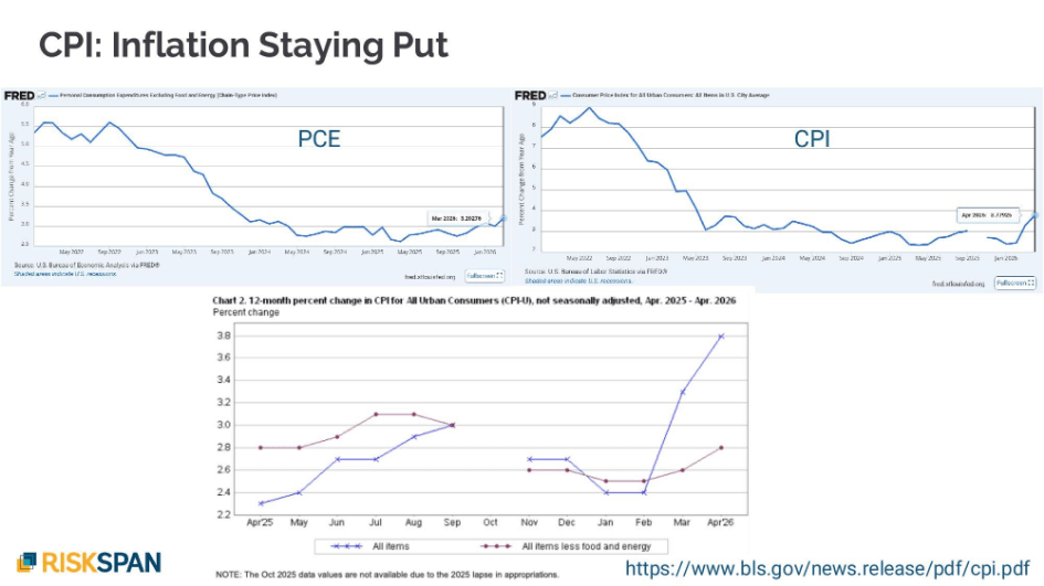
Figure 9: PCE Inflation (ex. Food & Energy) and CPI — Year-over-Year % Change
Home Prices — Stagnating, with Pronounced Regional Variation
National home price growth has slowed to near-zero. The Case-Shiller National Index showed approximately +0.67% year-over-year as of February 2026, while the 10-City Composite came in at +1.74%, suggesting urban markets are modestly outperforming. Regional divergence is pronounced: San Francisco has recorded negative price growth for approximately the past six months (-0.34% YoY), while New York remains solidly positive at +4.78%.
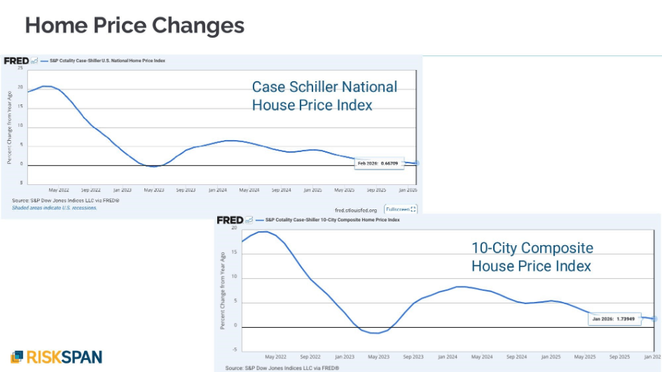
Figure 10: Case-Shiller National and 10-City Composite Home Price Indices — Year-over-Year % Change

Figure 11: Case-Shiller San Francisco and New York Home Price Indices — Year-over-Year % Change
Consumer Stress: Evidence from Credit Card Spending
This month’s call featured a deep dive into consumer financial stress, drawing on research from the Federal Reserve Bank of Boston. The analysis is particularly relevant to mortgage credit risk given evidence of rising delinquencies in FHA and Non-QM collateral.
Credit Landscape
Agency loans (excluding FHA) continue to show low delinquency rates with no significant deterioration. FHA, however, is exhibiting elevated delinquencies that remain high even after accounting for the trial modification policy introduced in October 2025, which holds more loans in delinquent states during the modification process. The Non-QM universe has also begun to show a rising delinquency trend over the past 12–18 months.
Boston Fed Analysis: Spending and Debt by Income Group
A study from the Federal Reserve Bank of Boston segments credit card behavior across three income cohorts and reveals a striking disparity between spending levels and outstanding balances:
- Low-income ($0–$39K): monthly spending ~$25B vs. revolving debt ~$80B — a 3x ratio; this group is primarily revolving rather than paying off balances
- Middle-income ($59K–$83K): spending ~$37B vs. debt ~$105B — also approximately a 3x ratio
- High-income ($121K+): spending ~$170B vs. debt ~$185B — roughly 1:1, consistent with transactor behavior (spend and pay off monthly)
Low- and middle-income households are therefore carrying roughly three months’ worth of spending as permanent revolving debt, at credit card APRs recently running around 23% on new issuances. Total credit card outstanding nationally has reached approximately $1.25 trillion.

Figure 12: Aggregate Credit Card Spending by Income Group, January 2015–May 2025 (Source: Boston Fed / Federal Reserve Y-14M)

Figure 13: Aggregate Credit Card Debt by Income Group, January 2015–April 2025 (Source: Boston Fed / Federal Reserve Y-14M)
Buy Now, Pay Later: An Untracked Risk
Buy now, pay later (BNPL) services have grown rapidly and appear to be used disproportionately by lower-income households. Because BNPL obligations are not reported to credit bureaus, they represent an invisible liability not reflected in standard debt figures. The team flagged this as a developing risk to monitor, particularly for its potential impact on borrower liquidity and mortgage performance in the FHA universe.
Summary
| Topic | Key Takeaway |
| Prepayment Model | Performing well overall; April discount speeds stable (turnover-driven); May premium speeds fell sharply on March rate sell-off and S-curve flattening |
| GNMA Performance | Discount speeds supported by turnover; premium speeds declined moderately but more resilient than conventional counterparts |
| Non-QM Credit Model | CM 7.1 beta in June; production release ~July 10; dedicated webinar in second half of June |
| Mortgage Rates | Freddie Mac at 6.51%; Mortgage News Daily at 6.65%; back to summer 2025 levels; sub-6.25% rate unlikely near-term |
| Fed Policy | No cuts expected in 2026; CME FedWatch shows meaningful probability of hike later in 2026 or early 2027 |
| Treasury Yields | 10-year up ~50 bps since February; 2-year up ~75–80 bps; consensus at ~4.82% by year-end |
| Inflation | CPI 3.8% YoY (April); core CPI 2.8%; PCE similarly elevated; well above 2% target |
| Home Prices | National ~+0.67% YoY; San Francisco negative; New York +4.78%; highly geography-dependent |
| Consumer Stress | Low/mid-income households revolving 3x monthly spending at ~23% APR; BNPL obligations add hidden risk; FHA and Non-QM delinquencies trending higher |
We continue to add additional analytics reports on the RiskSpan Platform. Please visit www.riskspan.com/request-access to request free access.
As always, please feel free to contact us to discuss or learn more.
AI is already disrupting parts of the U.S. labor market. The more contested question for residential mortgage investors is how and where. The dooms-day camp sees broad structural displacement where white-collar knowledge workers are replaced by AI agents. The optimists counter that AI makes workers more productive, that falling labor costs will expand demand leading to net employment gains. Both camps agree on one thing: the impact will not be uniform. Disruption will concentrate in pockets — specific occupations, metro centers, and income bands.
That specificity is precisely what makes this a mortgage credit problem. Local labor shocks have always transmitted to local housing markets through a familiar mechanism: income impairment reduces demand which pressures home prices, and price declines erode the collateral cushion that protects investors. What varies is the speed, the depth, and whether prices recover once the shock stabilizes.
Early indicators are consistent with the thesis. A Wall Street Journal analysis found the unemployment rate for recent college graduates ages 20–29 at 7.1% as of October 2024 — nearly double the 4.1% rate for the general population — with computer science graduates at 6.1% unemployment and computer engineering majors at 7.5%. The Federal Reserve of NY also published data showing labor market conditions worsened for recent college graduates at the end of 2025, with the unemployment rate climbing to about 5.7% in Q4 2025 — and underemployment rising to 42.5%, its highest level since 2020.
The occupations most exposed to AI displacement cluster in precisely the metros where high-balance prime mortgages are most concentrated, changing the traditional metrics that investors rely on for early warning. AI-driven labor disruption is not a macro thesis to be managed with national averages. While mortgage borrower occupation data is not complete or granular enough to drive AI job loss assumptions, property location data is. The risk needs to be identified, stress-tested, and monitored at a granular level — before it shows up in delinquency data.
The good news is that the data, models and historical reference points exist. With the growth of Non-QM lending, RTL and loan products that carry credit risk without an insurance wrapper, treating AI-driven labor disruption as a present-tense portfolio risk is not optional. To move from thesis to numbers, we ran a portfolio-level stress test on the universe of securitized Non-QM mortgages – starting with how AI exposure is measured at the local level.
Key Findings for investor consideration:
- AI labor disruption is expected to have a higher disproportional impact on white-collar professional jobs that are concentrated in certain “knowledge-work” centers.
- The largest job markets and the deepest credit pools are systematically the most AI-exposed, suggesting AI risk and portfolio risk overlap rather than diversify.
- Stress-testing the $196B universe of securitized Non-QM mortgage loans shows the magnitude is meaningful: under an AI-driven stress scenario calibrated to GFC-level shocks but re-allocated to AI-exposed geographies, RiskSpan’s credit model projects universe-wide cumulative defaults to nearly double and losses more than quadruple.
- Securitized deals benefit from built-in geographic diversification, which dampens the absolute impact across deals. Whole-loan investors, who construct their own geographic mix, face concentration risk that accumulates silently if exposure isn’t an explicit input into selection and surveillance.
- Act now — put the infrastructure in place to use granular data to monitor unemployment, HPI and loan performance and apply scenarios where relevant.
Measuring AI Exposure at the Local Level
Leveraging research published by the Brookings Institution, RiskSpan used their geographic AI exposure scores as the foundation for a credit stress scenario. The resulting county- and metro-level scores follow a similarly clear geographic pattern to that published by Brookings. Highly educated, high-paying knowledge-work centers — Santa Clara (42.8% exposure), King County WA, New York County, DC, Boston — show the highest exposure. Smaller industrial and rural counties score considerably lower. As a sanity check on the methodology, we aggregated and plotted state-level AI exposure against the share of each state’s adult population with a bachelor’s degree or higher (a well-understood proxy for knowledge-work concentration). The two track closely, which is the result one would expect — it confirms the Brookings measure is capturing what it intends to and isn’t producing arbitrary geographic rankings.

Unlike earlier automation, generative AI concentrates in exactly the metros that house the largest mortgage markets: as the chart below shows, the most AI-exposed MSAs are also among the deepest non-agency RMBS markets.

One important caveat before moving on to how we used this data. As Brookings is careful to note, “‘exposure’ does not speak only to the displacement of workers; it also may involve their ‘augmentation’ through rapidly improving AI tools.” The same coder whose role is highly exposed could be made dramatically more productive rather than displaced; the same financial analyst could spend less time on rote modeling and more on judgment-intensive work. Whether exposure plays out as net displacement, net augmentation, or some mix will vary by occupation, employer, and how quickly the technology evolves. For purposes of this exercise, we focus on the displacement story: the scenario where AI exposure translates into labor market shocks that transmit to housing markets and mortgage credit. That’s not the only possible outcome, but it’s the one investors need to be prepared for.
Translating that exposure into a portfolio-level credit stress test on the Non-QM universe, the largest segment of the non-agency RMBS market, required two steps.
Step 1: Construct an AI-driven stress scenario calibrated to the GFC.
Rather than forecast AI displacement magnitude — a genuinely uncertain exercise — we sized the stress to a known reference point: the total HPI decline and unemployment increase observed during the GFC. The GFC offers a useful calibration episode because the empirical relationship between local unemployment shocks and HPI declines is strong and well-documented, regardless of which direction the causation primarily ran. The chart below shows that relationship across MSAs — a clear negative slope linking the spike in unemployment rates to the depth of the HPI decline.

The critical observation for our purposes is what happened in 2008: the metros most exposed to AI today (DC, Boston, San Francisco, Seattle) cluster toward the middle of that scatter plot. They experienced more moderate impacts than the hardest-hit metros, because the speculative and underwriting excesses that drove the GFC were concentrated elsewhere — Las Vegas, Phoenix, Miami, the Inland Empire. An AI-driven shock would invert that geography.
We took the GFC’s national-level shock magnitudes and redistributed them, concentrating the stress in MSAs with high AI exposure. Starting from Brookings’ occupation-level AI exposure scores rolled up to MSA and state-level, we scaled both the unemployment and HPI shocks to each MSA in proportion to its AI exposure share. The result is a per-MSA stress profile that adds up to GFC-magnitude pain at the national level but lands very differently on the map.
The chart below translates that scaling into implied HPI shock magnitudes across the metros where non-agency RMBS exposure actually sits. The metros at the bottom end of both axes (high portfolio balance and severe implied HPI shock) are where the AI thesis would hit hardest if it materializes.

Step 2: Run the loan universe through two scenarios.
We took the $196B universe of Non-QM mortgage loans (~500K loans across 810 active Non-QM deals as of April 2026) and ran these loans through RiskSpan’s proprietary credit model under two scenarios: a baseline and the combined AI-driven Unemployment + HPI stress scenario described above. Every loan received a projected cumulative default rate and cumulative loss rate under each scenario, isolating the AI-driven impact at the loan level.
Findings
Under the AI-driven combined stress scenario, universe-wide cumulative defaults nearly double (3.6% → 7.4%) and cumulative losses more than quadruple (0.5% → 2.2%). The steeper loss response reflects the familiar non-linearity between defaults and severities under HPI stress. The mechanism behind those aggregate numbers becomes clearer when you look at it geographically.
Finding 1 — AI exposure drives MSA-level credit performance.
This finding is by construction — we built the stress scenario by re-allocating shocks to AI-exposed MSAs, so the model output should track AI exposure. The MSA-level chart confirms it does. MSAs at the high end of AI exposure (DC, San Francisco, Boston, Seattle) see over an 8% percentage point (pp) increase in cumulative defaults compared to MSAs at the low end. Riverside, near the lower end of the AI exposure range at just under 30%, sees only a 2.6% pp increase in cumulative defaults. There’s MSA-specific noise from collateral mix, but the geographic risk concentration the AI thesis predicts shows up cleanly in the model output. This is the core mechanism: re-allocate the stress to AI-exposed geographies, and the credit impact tracks the re-allocation.

Finding 2 — The aggregate impact is shaped primarily by leverage.
Decomposing the universe results by current LTV bucket explains where the headline numbers come from. The first thing worth noting is what the LTV distribution looks like: less than 5% of total non-QM balance sits above 80% LTV, and roughly half is below 60%. That’s a meaningfully larger equity cushion than the borrower base of the mid-2000s, when the proliferation of low- and no-down-payment products left investors with thin protection against any HPI decline. Today’s Non-QM universe starts the AI stress scenario with a lot more skin in the game.
Within that distribution, stress impact scales monotonically with leverage, exactly as one would expect: low-LTV loans (≤40%) see a 1.3pp increase in defaults (from 0.96% to 2.24%), while high-LTV loans (>80%) see a 6.7pp increase (from 5.97% to 12.62%), though the relative impact on cumulative defaults is broadly stable across LTV buckets, with defaults about doubling in each bucket. The same pattern holds for losses, where the highest LTV buckets see losses rise by over 3pp under stress versus 0.16pp for the lowest LTV bucket. FICO declines slightly as LTV increases (from 756 for the lowest LTV bucket to 745 for the highest), so the projected cumulative default differences across LTV buckets are driven, at least partly, by underlying borrower credit as well.

Finding 3 — Deal-level concentration matters, but only in relative terms.
When we rolled up by deal rather than by MSA, the picture got more interesting. The absolute (pp) impact across deals shows essentially no relationship with the deal’s AI exposure share — high-AI-exposure deals don’t show systematically larger pp increases. But the relative impact (stress / base − 1) is clearly correlated with AI exposure.
One plausible explanation is that deal-level base default rates vary widely based on traditional credit characteristics — LTV mix, FICO mix, doc type (Full Doc vs. DSCR vs. Bank Statement), occupancy. That variation in base rates may be dominating the AI signal in absolute terms while leaving it visible on a relative basis. Either way, the relative measure is the cleaner lens for isolating AI exposure’s marginal contribution to deal-level risk.
There’s also a more reassuring story embedded in these charts, at least for securitized mortgage assets. Compare the deal-level scatter to the MSA-level scatter and you’ll notice the deal-level points cluster in a meaningfully narrower range — both on the AI exposure axis (X) and on the impact axis (Y). That tighter clustering is geographic diversification at work: even the most AI-concentrated deal in the universe pulls in loans from enough different MSAs that its blended AI exposure sits closer to the universe average than the most exposed individual MSA does. Diversification within deals is doing what it’s supposed to do — dampening the variance of outcomes — even though the unit of analysis is smaller than an MSA. The magnitude of the differential across deals is bounded by how concentrated any individual issuer is willing to get.


The implication for whole-loan portfolios is sharper. Whole-loan investors don’t get the benefit of pre-built deal diversification — they’re constructing their own geographic mix one loan or pool at a time, and concentration risk accumulates silently if it isn’t an explicit input into selection and surveillance. AI exposure is one such risk, and a relatively new one, but it sits alongside more familiar concentrations — natural disaster exposure, regional employment dependencies, single-industry metros — that warrant the same lens. The toolkit is the same in each case: granular geographic data, stress scenarios calibrated to defensible reference points, and loan-level credit modeling. Whether the goal is initial portfolio construction or ongoing surveillance of a seasoned book, the ability to identify these concentrations early — before they show up in delinquency data — is what separates active risk management from passive observation.
What This Means for Investors
History offers instructive analogies including the energy-patch metros of the mid-2010s when oil prices collapsed — Houston, Oklahoma City, and Calgary experienced home price corrections in the range of 5 to 15 percent. Regional manufacturing declines showed a similar story over a longer time period — the long contraction of auto-sector employment in Detroit, for example, played out in local housing markets over years while national HPA remained positive. In neither case did the national trend warn you that specific MSAs were in distress.
Acting now means two things in practice. The first is tracking — building the early-warning infrastructure before you need it. That means monitoring MSA-level unemployment, not just the national rate; watching labor force participation shifts; and tracking occupational mix changes in the markets where your collateral is heaviest. These indicators move before delinquency does. The second is scenario preparation — running stylized AI displacement shocks against the portfolio today using MSA-level or county-level HPA overrides and occupational exposure overlays. The goal is not a forecast but rather a map of your exposure — which corners of the portfolio are most sensitive to particular labor market stress, and what the loss distribution looks like if the more adverse scenarios begin to materialize. That map is worth building now, while the cost of being wrong about the timing is low.
RiskSpan is releasing a new Non-QM-specific credit model in the coming weeks, estimated directly on Non-QM performance data and designed around the underwriting features (DSCR, bank statement, expanded LTV) that distinguish these segments. Re-running this scenario and other stress scenarios on the new model is on the near-term roadmap and may sharpen some of the findings reported here. For investors who want to evaluate their own exposure, the analytical infrastructure described here can be applied to specific portfolios on request.
Note: The Brookings Institution has been tracking AI’s labor market impact since 2019. A 2024 Brookings piece analyzed data from OpenAI to measure occupational AI exposure as the share of tasks where AI could reduce human completion time by at least 50%. AS one would expect, the cognitive/manual divide is evident in the rankings, with computer and mathematical work atop the list at 75% while construction sits at the bottom at 5.6%.
Their 2025 piece extends that work to geography by multiplying each occupation’s exposure rating by its share of local employment in each county or metro, then aggregating. Counties with large workforces in highly exposed occupations (software developers, financial analysts, lawyers, marketing professionals) score higher than those whose employment skews toward construction, agriculture, or in-person services.
Key References:
Generative AI, the American worker, and the future of work | Brookings
There Is Now Clearer Evidence AI Is Wrecking Young Americans’ Job Prospects – WSJ